RF pulses — watch the spins
dmipy-sim represents an RF pulse the same way it represents a gradient: as the actual
waveform you play on the coil. A Waveform is the gradient \(G(t)\); a B1Pulse
is the complex transmit field
on a uniform raster. The magnitude sets the nutation rate \(\gamma|B_1|\); the phase sets the rotation axis. Everything else — a 90°, a 180°, a slice-selective sinc — is just a shape, and the forward plays whatever you hand it.
The forward has no intent
bloch_simulate doesn't know a pulse is "excitation" or "refocusing" — it integrates the
Bloch equation for the \(B_1(t)\) you give it and reports what the magnetisation does. The
intelligence — choosing a pulse to hit a goal under hardware limits — lives one layer up, in
dmipy-design's RF optimiser. This page is the forward; that page is the
optimiser in front of it.
The zoo: shapes are conveniences on top of \(B_1(t)\)
from dmipy_sim.rf import B1Pulse, bloch_simulate, slice_profile

# constructors are conveniences — the ground truth is always the B1(t) array
exc  = B1Pulse.hard(flip_deg=90,  duration=1e-3, dt=1e-6)          # rectangular 90°
inv  = B1Pulse.hard(flip_deg=180, duration=1e-3, dt=1e-6)          # rectangular 180°
sinc = B1Pulse.windowed_sinc(90, 2.56e-3, 1e-5, time_bw=4)         # slice-selective
free = B1Pulse.from_samples(my_complex_b1_array, dt=1e-5)          # anything at all

exc.peak_b1, exc.sar_proxy, exc.nominal_flip_deg   # amplitude / SAR / area
inv.is_deliverable("ge_signa_premier_3T")          # vs the scanner catalogue
Excitation vs inversion
Hand the forward a 90° and a 180° hard pulse of the same duration — same code path, different area. The 90° tips the magnetisation from \(+z\) into the transverse plane (signal you can read); the 180° drives it through to \(-z\) (inversion, the basis of a refocusing or an IR prep).
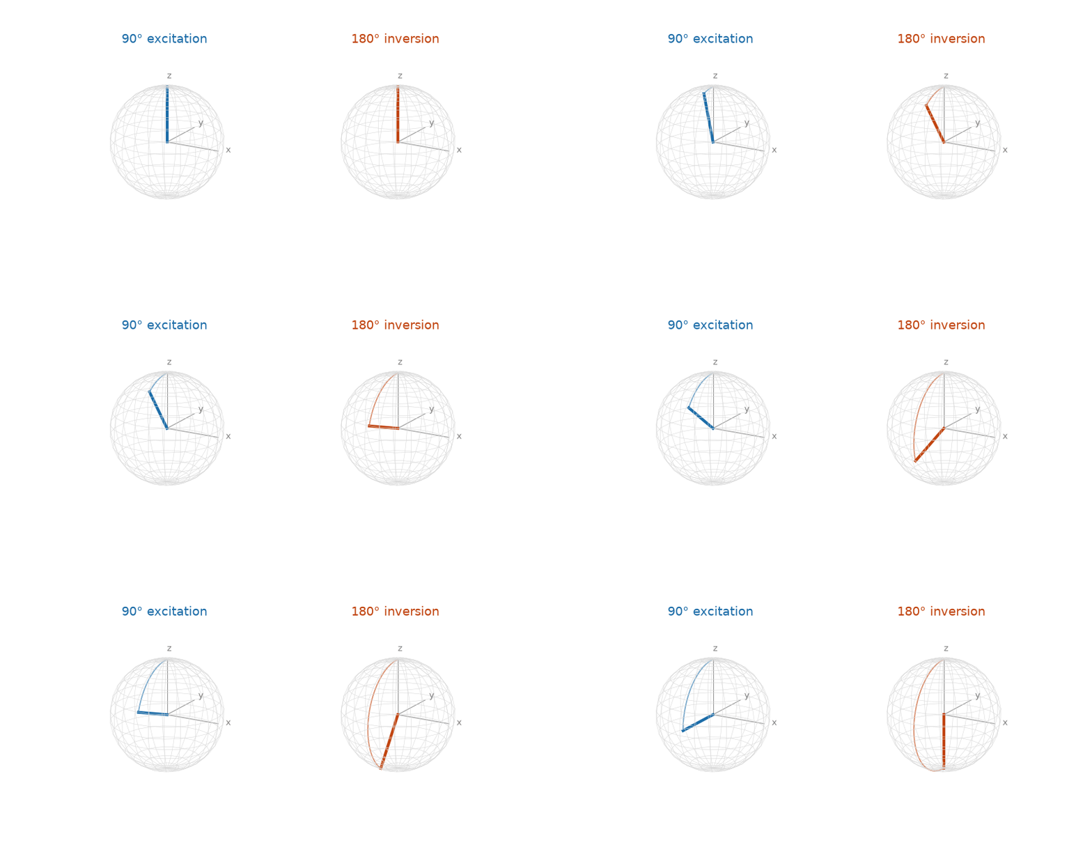
_, _, hist = bloch_simulate(exc, df_hz=0.0, return_history=True)   # M at every raster step
Mxy, Mz = bloch_simulate(inv, df_hz=0.0)                           # end-state only
Slice selectivity and the frequency dual
Under a slice-select gradient, a spin at position \(z\) sees an off-resonance \(\tfrac{\gamma}{2\pi}G_{ss}z\), so the excitation profile in space is (small-tip) the Fourier transform of the \(B_1\) envelope. A rectangular hard pulse therefore excites a sinc in frequency/space (ripples everywhere — no selectivity); a windowed sinc pulse excites a near-rectangular slice.
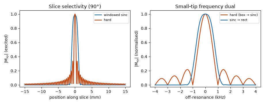
z, Mxy, Mz = slice_profile(sinc, slice_gradient=20e-3, positions_m=z) # T/m, metres
Refocusing trains: Carr-Purcell vs Meiboom-Gill
The phase of a pulse is its rotation axis — and that choice can make or break an echo train. In a CPMG train the 180° pulses are never exactly π (here B1⁺ = 0.8 makes them ~144°), and the axis decides what happens to that error:
- Carr-Purcell — 180ₓ, axis perpendicular to the transverse magnetisation. The flip error tips spins out of plane a little each echo and the errors accumulate — the train collapses.
- Meiboom-Gill — 180_y, axis parallel to the magnetisation (the 90ₓ left M along ∓y). The error on an odd echo is undone on the next even echo — the train is self-correcting.
Same imperfect pulse, opposite outcome, from one 90° phase shift. This is just B1Pulse phases
through the forward:
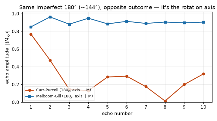
refoc_cp = B1Pulse.hard(180, 4e-3, 1e-5, phase_deg=0)    # axis ⟂ M  → errors accumulate
refoc_mg = B1Pulse.hard(180, 4e-3, 1e-5, phase_deg=90)   # axis ∥ M  → self-correcting
Robust refocusing: a small taxonomy
A hard 180° only inverts properly at the nominal transmit strength. There are three classic ways to make it B1-robust, and dmipy plays all of them through the same forward:
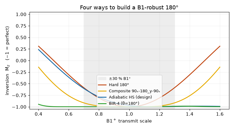
- Composite (
90ₓ-180_y-90ₓ) — robustness from a designed sequence of simple rotations; build it by concatenating hard segments with different phases. - Adiabatic HS — robustness from a continuous frequency sweep: the magnetisation follows
the effective field. This is what
design_refocusing_rfproduces. - BIR-4 — an adiabatic pulse that rotates by any angle B1-insensitively (below).
Each is a first-class B1Pulse constructor:
composite = B1Pulse.composite([(90, 0), (180, 90), (90, 0)], dt=1e-5, peak_b1=15e-6)
adiab     = B1Pulse.adiabatic_hs(6e-3, 1e-5, peak_b1=19e-6, mu=2.0)   # HS full passage
The exotic: BIR-4, a B1-insensitive rotation by any angle
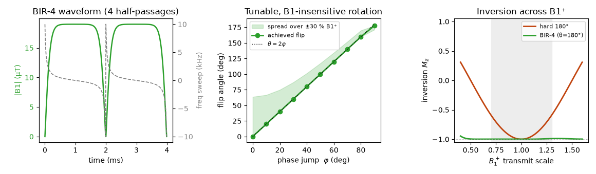
BIR-4 (B1-Independent Rotation, 4 segments; Garwood & Ke 1991) is built from four adiabatic half-passages with an alternating frequency sweep and two phase jumps. Where an adiabatic full passage can only invert, BIR-4 rotates by an arbitrary angle set by the phase jump (\(\theta \approx 2\varphi\)) — and does so B1-insensitively. It's the most robust refocusing element here, flat across the entire ±60% B1⁺ range:
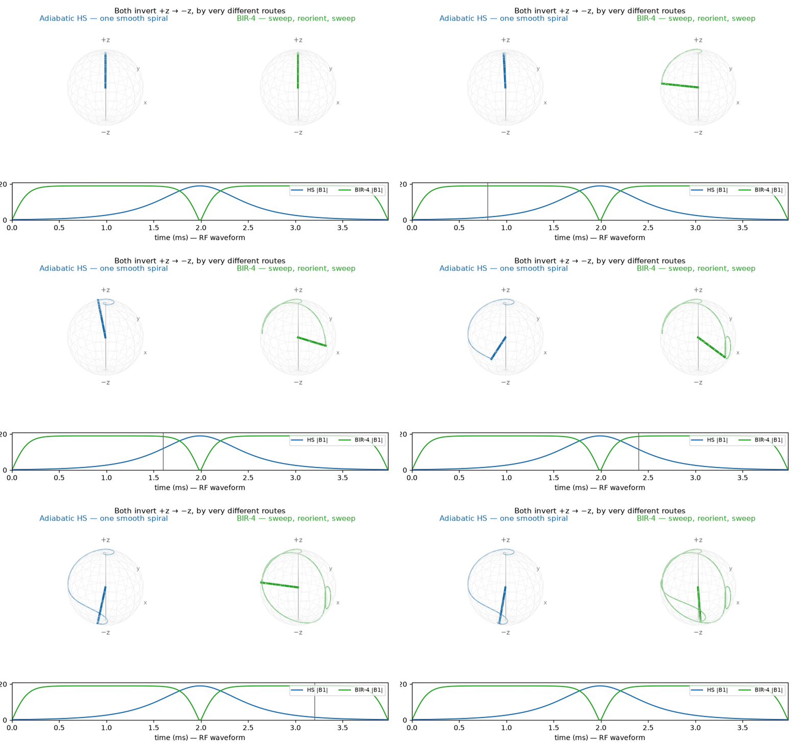
Both the adiabatic HS and BIR-4 invert \(+z \to -z\), but by very different routes on the Bloch sphere — the HS is one smooth spiral, while BIR-4 sweeps out toward the transverse plane, is reoriented at each of its two phase jumps, and only then lands at \(-z\). You can read the four-segment structure straight off the trajectory (and the double-hump \(B_1(t)\) below):
bir4 = B1Pulse.bir4(flip_deg=180, duration=4e-3, dt=1e-5, peak_b1=19e-6) # tunable rotation
Every pulse on this page — excitation, refocusing, slice-selective, CPMG, composite, adiabatic,
BIR-4 — is the same B1Pulse object through the same Bloch forward. dmipy-sim provides them
all as constructors (hard, windowed_sinc, adiabatic_hs, adiabatic_half_passage, bir4,
composite); the optimised pulses come from dmipy-design, which can warm-start
its optimiser from any of these — e.g. design_refocusing_rf(warm_start=B1Pulse.bir4(...))
refines a BIR-4 against your exact B1⁺/off-resonance ensemble.
The forward in full
bloch_simulate integrates over an ensemble — off-resonance df_hz × transmit scale
b1_scale both broadcast — with optional T1/T2 relaxation and a full return_history. That
ensemble is exactly what the refocusing-RF optimiser scores against when it
designs a \(B_1\)-robust 180°.
References
- Small-tip-angle theorem. Pauly J, Nishimura D, Macovski A. A k-space analysis of small-tip- angle excitation. Journal of Magnetic Resonance 81 (1989) 43–56. doi:10.1016/0022-2364(89)90265-5.
- Meiboom-Gill. Meiboom S, Gill D. Modified spin-echo method for measuring nuclear relaxation times. Review of Scientific Instruments 29 (1958) 688–691. doi:10.1063/1.1716296.
- Composite pulses. Levitt MH. Composite pulses. Progress in NMR Spectroscopy 18 (1986) 61–122. doi:10.1016/0079-6565(86)80005-X.
- BIR-4. Garwood M, Ke Y. Symmetric pulses to induce arbitrary flip angles with compensation for RF inhomogeneity and resonance offsets. Journal of Magnetic Resonance 94 (1991) 511–525. doi:10.1016/0022-2364(91)90137-I.
- Adiabatic pulses — review. Tannús A, Garwood M. Adiabatic pulses. NMR in Biomedicine 10 (1997) 423–434.