Magnetization transfer

✅ Operational in dmipy-sim

Magnetization transfer (MT) is a released effect in the Bloch Monte-Carlo engine — and it is not a two-pool rate law bolted onto the signal. Water spins physically stick to the myelin wall and exchange magnetization; the two-pool behaviour emerges from the walk. You can watch it happen below.

The picture in one paragraph

The water you image is mobile and gives the signal. Protons bound to macromolecules — myelin lipids and proteins — are all but invisible on their own: their \(T_2\) is a few microseconds, so any signal they carry dephases before you can read it. But the two pools trade places. A free water spin can bind to the wall, sit in the dark bound pool for a while, and come back. That trade is magnetization transfer. Because it happens at the wall, its rate scales with the wall area a spin sees — the same surface-to-volume ratio \(S/V\) that drives surface relaxivity.

Watch the burn-in

A real dmipy-sim walk — the same binding law the engine runs (dmipy_sim.mt), rendered by docs/media/fig_mt_burnin.py.

• Left — the walk. One myelinated cylinder in a small periodic cell. Each dot is a water walker: teal while free, amber while bound to the myelin. Free walkers random-walk; when one reaches the myelin surface it may stick (a chance proportional to how hard it hits — the boundary local time), freeze there for a dwell time, then release back into free diffusion.
• Right — the bound pool filling. The fraction of walkers currently bound. It starts at zero — a fresh simulation begins with every spin free — and climbs as binding outpaces release, until the two balance at the thermal equilibrium \(f_b = k_f/(k_f+k_r)\) (dashed line). Nothing imposes that value: it is simply where the walk settles, and it lands on the analytic equilibrium.

How it works — emergent wall sticking

Every effect in the equilibrium above is a consequence of spins sitting on the wall, not a prescribed kernel:

• Binding (\(k_f\)): a walker that contacts the myelin sticks with probability \(\min(1,\,2\,(\kappa_{\mathrm{MT}}/D)\,\ell)\), where \(\ell\) is the boundary local time of the hit — the exact same wall-contact statistic surface relaxivity uses. So the forward rate inherits the geometry, \(k_f = \kappa_{\mathrm{MT}}\,(S/V)\).
• The dark bound pool: a bound walker is frozen in place and carries the myelin's ultra-short \(T_2\), so its transverse magnetization dephases almost instantly — it is MR-invisible while stuck.
• Release (\(k_r\)): it stays bound for a dwell time drawn from \(k_r = 1/\tau_{\text{dwell}}\), then rejoins the free walk.

Run one MT walk and the Z-spectrum, MTR, and exchange all fall out of these three rules — there is no super-Lorentzian lineshape or Bloch–McConnell rate matrix anywhere in the forward pass.

Why the burn-in is required (and enforced)

The animation shows the catch directly: a fresh walk starts with the bound pool empty, which is not the state a real acquisition sees — in tissue the pools sit at their thermal equilibrium before the first pulse. If you fired the sequence at \(t=0\) the bound pool would still be filling, and the signal would be biased.

So dmipy-sim runs an RF-off, gradient-off burn-in first, letting binding and release equilibrate until the occupancy plateaus at \(k_f/(k_f+k_r)\) — the right panel — and only then fires the actual sequence. It also checks that the occupancy has equilibrated before firing: an under-burned run is flagged rather than silently returning a biased signal. (The characteristic burn-in time is \(\tau = 1/(k_f+k_r)\); the engine burns in for several \(\tau\).)

Two rates, one wall — the coherence-gating split

MT is the one effect the coherence gate splits, because it has two pathways on opposite sides of it. While the magnetization is transverse, the short-\(T_2\) bound pool drains the free pool during encoding — this is the \(k_f\) above — and it enters the apparent transverse rate in exactly the surface-relaxivity form:

\[ \frac{1}{T_2^{\mathrm{app}}} = \frac{1}{T_2} + \rho_2\,\frac{S}{V} + R_2' + k_f . \]

A separate longitudinal saturation-transfer pathway exchanges \(M_z\) in both coherence states, so it survives longitudinal storage:

\[ \frac{1}{T_1^{\mathrm{app}}} = \frac{1}{T_1} + \rho_1\,\frac{S}{V} + k_{\mathrm{MT}}^{\parallel} . \]

A stimulated echo therefore pauses MT's transverse face during the mixing time but still pays the longitudinal one — so MT gains less from gating than the purely transverse channels (surface relaxivity, susceptibility), and the longitudinal term is left as a residual, non-gated confound.

The third observable — the Z-spectrum

Diffusion and relaxation can't tell an MT wall from a plain surface-relaxivity wall — both simply attenuate. The Z-spectrum can. Sweep a saturation pulse across a range of frequency offsets from the water line and record how much longitudinal signal survives: the narrow free-water line is only touched near resonance, but the bound pool's ultra-short \(T_2^{b}\) lets it keep absorbing across a broad offset range — so the free signal stays depressed far off-resonance. That off-resonance dip is something only a bound pool can make; it is MT's fingerprint, and the observable that separates the transfer share of a wall's reactivity from surface relaxivity.

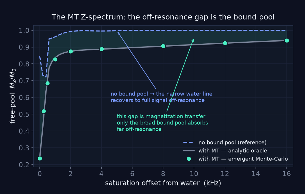
One call runs it — dmipy_sim.emergent_z_spectrum(offsets, geometry, …) does a real forward walk at each offset — and the emergent points land on the analytic two-pool oracle (line) to the Monte-Carlo noise floor, the same agreement the burn-in buys, now across the whole spectrum.

The two-pool system we validate against

That oracle is a full two-pool Bloch–McConnell model — and full is the point: it carries both pools' complete magnetization — free \(a\) and bound \(b\), transverse and longitudinal — and lets the bound pool's real short \(T_2^{b}\) do the dephasing. It uses no super-Lorentzian lineshape and no phenomenological RF-absorption rate \(R_{\mathrm{rfb}}\); the broad off-resonance saturation emerges from the short-\(T_2^{b}\) spin. For RF of nutation rate \(w_1=\gamma B_1\) about axis \(\phi\), off-resonance \(\Delta\omega_p\), and exchange \(k_f\) (free→bound) / \(k_r\) (bound→free):

\[ \begin{aligned} \dot M_x^{p} &= -R_2^{p}M_x^{p} - \Delta\omega_p\,M_y^{p} + w_1\sin\phi\,M_z^{p} - k^{p}_{\text{out}}M_x^{p} + k^{p}_{\text{in}}M_x^{q}\\ \dot M_y^{p} &= +\Delta\omega_p\,M_x^{p} - R_2^{p}M_y^{p} - w_1\cos\phi\,M_z^{p} - k^{p}_{\text{out}}M_y^{p} + k^{p}_{\text{in}}M_y^{q}\\ \dot M_z^{p} &= -w_1\sin\phi\,M_x^{p} + w_1\cos\phi\,M_y^{p} - R_1^{p}\big(M_z^{p}-M_0^{p}\big) - k^{p}_{\text{out}}M_z^{p} + k^{p}_{\text{in}}M_z^{q} \end{aligned} \]

for \((p,q)=(a,b)\) with \((k^{p}_{\text{out}},k^{p}_{\text{in}})=(k_f,k_r)\) and \((p,q)=(b,a)\) with \((k_r,k_f)\); \(M_0^{b}=M_0^{a}\,k_f/k_r\) by detailed balance. Exchange couples all three components of each pool — including the bound transverse ones \(M_x^{b},M_y^{b}\). The reduced 4-equation qMT model (drop \(M_x^{b},M_y^{b}\) and replace their RF response with a lineshape-based \(R_{\mathrm{rfb}}\) on \(M_z^{b}\)) is deliberately not used; and neither this ODE nor any lineshape enters the forward walk, where the two-pool behaviour is emergent. The analytical inverse (dmipy-fit) counterpart follows.