B1-robust refocusing RF

The rest of dmipy-design works in the instant-pulse approximation — an ideal hard 180° that inverts every spin perfectly, everywhere. A real refocusing pulse does not. Across a head the transmit field \(B_1^+\) varies by tens of percent, so a hard 180° that is exactly π at the coil centre becomes a 126° at \(B_1^+=0.7\) and a 234° at \(B_1^+=1.3\) — the off-nominal spins are never properly flipped, the spin echo built on them is incomplete, and that is signal you simply lose.

The standard, scanner-deliverable fix is an adiabatic pulse: sweep the RF frequency slowly through resonance while the amplitude rises and falls, and — provided the sweep is slow enough (the adiabatic condition) — the magnetisation follows the effective field from +z to −z regardless of the exact \(B_1^+\). design_refocusing_rf builds the classic hyperbolic-secant (HS) adiabatic full passage (Silver, Joseph & Hoult 1985) tuned to your hardware, then refines it with a short optimal-control (GRAPE) pass — the HS pulse is the good initial guess that keeps the refinement physical.

It is the RF analogue of the NOW gradient box: design a deliverable waveform that meets a physical spec under the real hardware limits — here \(B_1(t)\) instead of \(G(t)\).

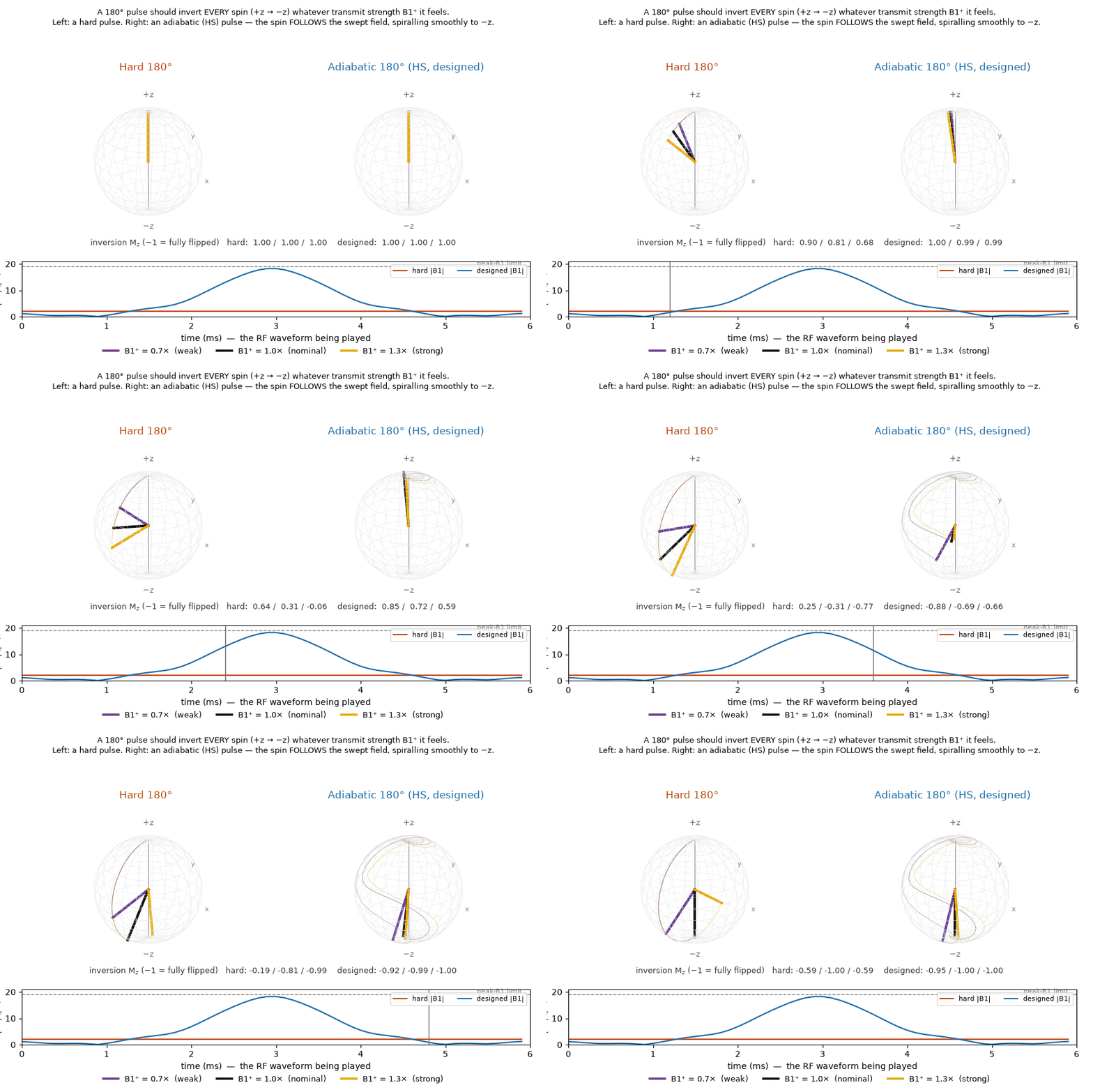
New to RF pulses? The RF pulses — watch the spins page (dmipy-sim) shows what a \(B_1(t)\) envelope is and how the Bloch forward plays any pulse — this page designs one.

Idealized vs real refocusing

Idealized theory	Real hardware
instantaneous, perfect π everywhere	finite-duration pulse; a fixed-flip pulse's angle scales with \(B_1^+\)
single on-resonance spin	a spread of static off-resonance (\(B_0\), susceptibility)
unbounded RF	peak \(B_1\) cap (body-coil hardware limit) and SAR (heating)
any shape	bandwidth / RF slew limited by the transmit chain

Why the adiabatic pulse is robust — and how it's scored

An adiabatic pulse doesn't try to hit exactly 180°; it makes the effective field sweep from far above resonance, through zero, to far below, and the magnetisation is dragged along with it. Change \(B_1^+\) and the sweep is a little faster or slower, but as long as it stays adiabatic the spin still arrives at −z — that is the source of the robustness, and why every trajectory above is a smooth spiral rather than a delicate balance.

The figure of merit is the crushed spin-echo refocusing efficiency

\[\eta = \tfrac12\,(1 - M_z) \in [0,1],\qquad M_z = \text{the pulse acting on } +z,\]

(\(\eta = 1\) for a perfect inversion, \(|\beta|^2\) in Shinnar–Le-Roux terms). It is a per-spin scalar, averaged over the \((B_1^+ \times \text{off-resonance})\) ensemble — so every spin must genuinely invert; it cannot be gamed by cross-spin phase cancellation.

The design maximises \(\langle\eta\rangle\) through the Bloch equation in two stages: first it picks the HS sweep parameter \(\mu\) (and, under a SAR cap, the amplitude) — a robust, physical starting pulse; then a GRAPE-style refinement optimises a few smooth correction modes of the full waveform, warm-started from that pulse. Because it starts in the adiabatic basin and the corrections are band-limited, the result stays a smooth deliverable spiral — it does not wander into a non-physical optimum the way a free-form search from a cold start does. (A generic optimiser with no good initial guess is exactly what fails here; the adiabatic pulse is the initial guess.) The refinement typically buys a little efficiency and peak-\(B_1\) headroom at equal SAR.

Deliverability — and the price of robustness

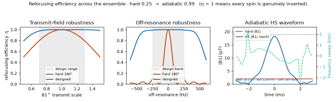
The amplitude is set to the deliverable peak (\(A_0 = B_1^{\max}\) — adiabaticity improves with amplitude, so you spend the coil's full peak), and the sweep bandwidth is chosen to cover the off-resonance band. Adiabatic pulses are power-hungry: following the field robustly costs RF energy — here ≈17× the SAR of a minimal hard 180°. sar_headroom caps that (as a multiple of the hard-180° energy) by lowering \(A_0\); left None the design is peak-limited (most robust) and reports the SAR it spent.

Limit	RF analogue of	Role
peak \(B_1 = A_0 \le B_1^{\max}\)	gradient amplitude box	hard hardware ceiling
SAR \(\propto \int\lvert B_1\rvert^2 dt\)	gradient heat limit	the price of adiabaticity

Use it

from dmipy_design import design_refocusing_rf

d = design_refocusing_rf(
    rf_duration=6e-3, dt=1e-4,      # 6 ms pulse on a 100 µs RF raster
    B1_max=19e-6,                   # GE SIGNA Premier body coil ≈ 19 µT (hard peak limit)
    sar_headroom=None,              # peak-limited (most adiabatic); or e.g. 8.0 to cap SAR
    b1_range=(0.7, 1.3), n_b1=7,    # ±30 % transmit inhomogeneity to invert across
    off_resonance_hz=250.0, n_off_resonance=7,   # ±250 Hz band the sweep must cover
    refine=True,                    # GRAPE refinement from the HS warm start (default)
)

d.refocusing_efficiency        # ensemble-mean η (0–1); 1 = every spin inverted
d.refocusing_efficiency_hard   # same metric for a plain hard 180° — the baseline
d.B1                           # complex B1 envelope, Tesla
d.mu, d.beta, d.bandwidth_hz   # the adiabatic (HS) backbone parameters
d.refined                      # True if the GRAPE pass improved on the HS template
d.peak_B1, d.sar_ratio         # delivered peak and SAR (× hard-180°)

Peak-limited on a 19 µT body coil, the hard 180° refocuses only η = 0.25 of the ±30 % / ±250 Hz ensemble; the HS adiabatic pulse reaches η = 0.99 — every spin inverted — at 18.9 µT peak, a ≈1.3 kHz inversion band, for ≈17× the RF energy of a hard 180°. Same echo time, far more signal; the SAR is the honest cost of adiabaticity.

Pushing it: the optimiser at the edge

On an easy spec the adiabatic warm start is already near-perfect and the GRAPE pass barely matters. Push to a hard spec — invert across ±50 % B1⁺ and ±500 Hz on a 19 µT / 5 ms budget — and the layers separate: a hard 180° is hopeless (η = 0.14), the HS warm start does the heavy lifting (η = 0.91), and the GRAPE refinement squeezes out the last bit of efficiency while trimming peak-B1 (18.9 → 16.3 µT of headroom):

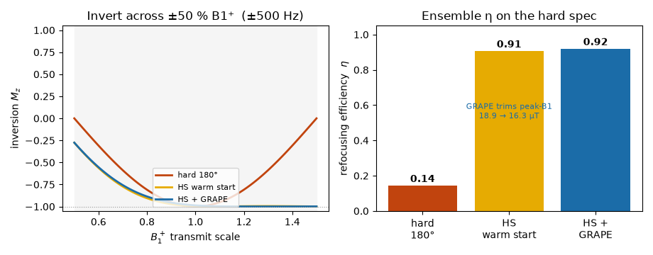
Left: inversion Mz vs B1⁺ across ±50% for a hard 180° (fails at the edges), the HS warm start, and HS+GRAPE (both flat near −1). Right: ensemble refocusing efficiency η — hard 0.14, HS 0.91, HS+GRAPE 0.92 — with GRAPE trimming peak-B1 from 18.9 to 16.3 µT.

This is dmipy-design's own optimiser working at the edge of what a 5 ms / 19 µT pulse can do — and a taxonomy of fixed robust pulses (adiabatic HS, BIR-4, composites; see RF pulses — watch the spins) is exactly the space of warm starts it refines from.

Refocusing vs inversion

An adiabatic full passage imparts a \(B_0/B_1\)-dependent phase, so as a refocusing pulse it is used as a matched pair (double adiabatic refocusing, e.g. LASER) to cancel that phase; the crushed-echo \(\eta\) here is the single-pass \(|\beta|^2\) refocusing coefficient. The pulse is designed in isolation (not coupled to the gradient); d.to_b1pulse() hands it to dmipy-sim's Bloch forward. NumPy/SciPy only.

References

The hyperbolic-secant adiabatic pulse and the crushed-echo / SLR refocusing efficiency are established; dmipy-design provides a NumPy/SciPy design + Bloch scoring, not an external library.

Hyperbolic-secant adiabatic pulse. Silver MS, Joseph RI, Hoult DI. Highly selective π/2 and π pulse generation. Journal of Magnetic Resonance 59 (1984) 347–351; and Phys. Rev. A 31 (1985) 2753. doi:10.1103/PhysRevA.31.2753.
Adiabatic pulses — review. Tannús A, Garwood M. Adiabatic pulses. NMR in Biomedicine 10 (1997) 423–434. doi:10.1002/(SICI)1099-1492(199712)10:8<423::AID-NBM488>3.0.CO;2-X.
Refocusing efficiency / SLR. Pauly J, Le Roux P, Nishimura D, Macovski A. Parameter relations for the Shinnar–Le Roux selective excitation pulse design algorithm. IEEE Transactions on Medical Imaging 10 (1991) 53–65. doi:10.1109/42.75611.