Generalized Kärger exchange (and NEXI)

Derivation note for the water-exchange models in dmipy_fit.signal_models.exchange_models — X0GeneralizedKarger wraps any two compartments with Kärger exchange. NEXI (Stick + Zeppelin with the tortuosity constraint) is just that general model with a pre-wired link, exposed as reference_models.nexi() — no special class. GPU forward functions live in dmipy_fit.jax.exchange_models_jax.

What it is. When a compartment boundary is permeable, spins cross between environments during the acquisition, so the signal is no longer a fixed-fraction sum of independent compartments. The Kärger model is the compartment-population description of that exchange: instead of tracking individual walkers (as the dmipy-sim Monte-Carlo does, where exchange emerges from wall-crossing events), it evolves the populations of the compartments under a coupled linear system. "Generalized" here means the two compartments are arbitrary dmipy-fit models — not hard-wired to a specific stick/ball pair.

The exchange system

For two exchanging compartments write the pathway amplitudes as \(\mathbf M(t)\in\mathbb R^2\) with initial populations \(M_{0,i} = f_i S_{0,i}\). The magnetisation evolves under a coupled linear ODE combining exchange, relaxation and diffusion,

\[ \frac{d\mathbf M}{dt} \;=\; \bigl[\,\mathbf K \;-\; \mathbf R(t) \;-\; \mathbf D(t)\,\bigr]\,\mathbf M , \]

where \(\mathbf K\) is the exchange-rate matrix

\[ K_{ij} = k_{ji}\ (i\neq j), \qquad K_{ii} = -\sum_{m\neq i} k_{im}, \]

\(\mathbf R(t)\) is the (diagonal) relaxation operator and \(\mathbf D(t)=\mathrm{diag}(q^2(t)\,D_i)\) the Gaussian diffusion-attenuation operator.

Detailed balance is on spin populations, not volumes

The exchange rates satisfy detailed balance of the spin populations:

\[ (f_i S_{0,i})\,k_{ij} \;=\; (f_j S_{0,j})\,k_{ji}, \]

where \(f_i\) is the geometric volume fraction and \(S_{0,i}\) the proton-density-weighted equilibrium signal. When proton densities are equal this reduces to the familiar \(f_i k_{ij} = f_j k_{ji}\) — but for compartments with different water content per unit volume (e.g. myelin water vs. free water) the product \(f_i S_{0,i}\) (the spin population), not the geometric volume, is what must balance. Getting this wrong biases the recovered exchange rate.

Spin-echo (PGSE): one interval, per-compartment \(T_2\)

In the instantaneous-RF limit the whole echo is a single transverse interval, so the ODE integrates to a matrix exponential,

\[ \mathbf M(\mathrm{TE}) \;=\; \exp\!\Bigl(\bigl[\mathbf K - \mathbf R_{T_2}\bigr]\,\mathrm{TE} \;-\; b\,\mathrm{diag}(D_i)\Bigr)\,\mathbf M_0, \qquad \mathbf R_{T_2}=\mathrm{diag}(1/T_{2,i}). \]

This is the standard two-Gaussian-compartment Kärger result with per-compartment \(T_2\) — each compartment relaxes at its own transverse rate while exchanging, and because \(\mathbf K\) and \(\mathbf R_{T_2}\) do not commute the coupling is not separable (you cannot factor exchange and relaxation apart).

Stimulated echo (PGSTE): \(T_1\) governs the mixing interval

In a stimulated-echo experiment the magnetisation is stored longitudinally during the mixing time \(T_M\). There, \(T_2\) no longer acts — \(T_1\) relaxation (and exchange) act instead — while \(T_2\) acts during each of the two transverse encoding lobes of duration \(\delta\):

\[ \mathbf M(\mathrm{TE}) = \tfrac12\, \underbrace{\exp\!\Bigl([\mathbf K-\mathbf R_{T_2}]\delta - \tfrac{b}{2}\mathrm{diag}(D_i)\Bigr)}_{\text{encode (transverse, }T_2)} \underbrace{\exp\!\Bigl([\mathbf K-\mathbf R_{T_1}]\,T_M\Bigr)}_{\text{store (longitudinal, }T_1)} \underbrace{\exp\!\Bigl([\mathbf K-\mathbf R_{T_2}]\delta - \tfrac{b}{2}\mathrm{diag}(D_i)\Bigr)}_{\text{encode (transverse, }T_2)} \mathbf M_0, \]

with \(\mathbf R_{T_1}=\mathrm{diag}(1/T_{1,i})\) and the \(\tfrac12\) stimulated-echo pathway factor. The consequence is physically important: PGSTE lets exchange act over a long \(T_M\) under \(T_1\) (typically \(\gg T_2\)), so the stimulated echo is more sensitive to slow exchange than a spin echo of the same diffusion weighting — and the two compartments' \(T_1\) values, not their \(T_2\), weight the stored populations.

Both forms extend to finite-RF pulses by inserting a per-interval matrix exponential for each pulse duration (with mixed \(T_1/T_2\) relaxation during the pulse) and evaluating the whole sequence as an ordered product of matrix exponentials — which is what exchange_models.py does (_karger_propagator_se, _karger_propagator_ste).

Validity, and where the Monte-Carlo takes over

The Kärger picture is a slow-exchange approximation. It holds when exchange is slow relative to both intra-compartment diffusion and relaxation,

\[ k_{ij} \ll D_i/R_i^2, \qquad k_{ij} \ll 1/T_{2,i}, \]

(\(R_i\) = compartment size). Outside that regime — in particular once \(k\,\Delta \gtrsim 1\) under typical PGSE timing — the Kärger formula systematically under-estimates exchange-induced signal change, and the dmipy-sim Monte-Carlo (where exchange is a genuine wall-crossing event along each trajectory, not a population rate) is the reference. Agreement between the analytical Kärger model and the MC in the slow regime is a consistency check on the interface, not a proof that either is correct outside it.

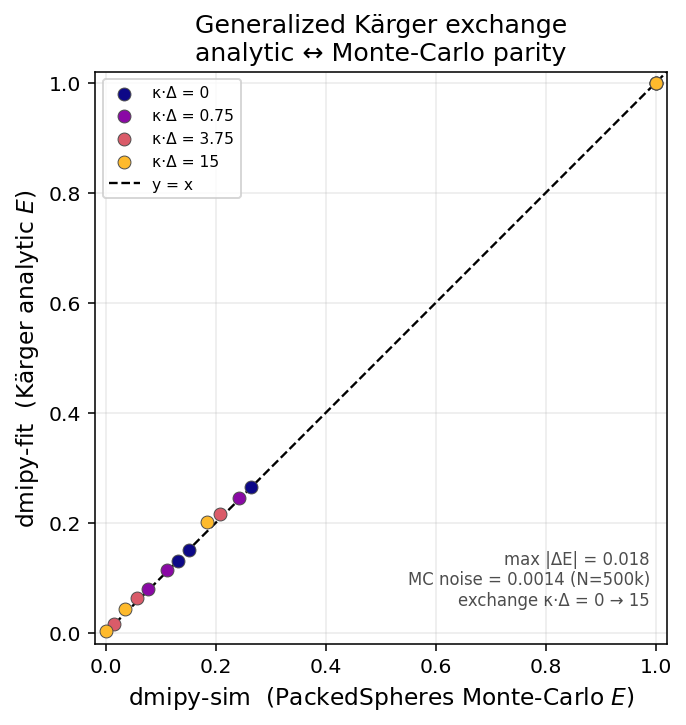
Within that regime the analytical X0GeneralizedKarger (GPA sphere + Ball) reproduces the dmipy-sim PackedSpheres Monte-Carlo across exchange strengths \(\kappa\,\Delta = 0 \to 15\) to within Monte-Carlo noise (max \(|\Delta E| = 0.018\), MC noise \(0.0014\) at \(N=500\text{k}\)) — every point on the identity line.

In code

from dmipy_fit.signal_models.exchange_models import X0GeneralizedKarger

# NEXI = Stick + Zeppelin + tortuosity, built via the general Kärger model:
from dmipy_fit.custom_optimizers.reference_models import nexi
model = nexi()

# or wrap ANY two compartments with Kärger exchange directly:
from dmipy_fit.signal_models.cylinder_models import C1Stick
from dmipy_fit.signal_models.gaussian_models import G1Ball
model = X0GeneralizedKarger(model_intra=C1Stick(), model_extra=G1Ball())

Per-compartment T2/T1 are picked up from the compartments when present (falling back to a global T2 or to no relaxation); the SE vs. PGSTE propagator is selected from the acquisition scheme (mixing time \(T_M\)). See also the GPA-for-arbitrary-waveforms derivation and Acquisition sequences.