OGSE spectral design

Why frequency, not just b

Two waveforms can have the identical b-tensor and still probe different tissue. PGSE and OGSE (oscillating-gradient spin echo) are both linear encodings — same b-tensor — yet OGSE reports on shorter length scales. The distinguishing quantity is spectral: to first order the diffusion attenuation is

\[ \ln S \;\approx\; -\int_0^\infty D(\omega)\,\lvert \tilde q(\omega)\rvert^2 \, d\omega, \]

where \(\tilde q(\omega)\) is the Fourier content of the encoding wavevector \(q(t)=\gamma\!\int s\,g\,dt\) and \(D(\omega)\) is the frequency-dependent diffusivity of the restricted/exchanging tissue. Sweeping the encoding frequency \(\omega\) is therefore a direct probe of restriction and exchange — which is exactly what OGSE is for. The b-tensor alone is blind to it.

Designing to a spectrum

dmipy-design treats the spectrum as a first-class design target rather than assuming a pure, monochromatic oscillation:

• spectral_freq=f drives the RMS encoding frequency to f — an OGSE-like oscillating waveform, for any b-tensor shape — using a differentiable, FFT-free constraint (\(f_\mathrm{rms} = \tfrac{1}{2\pi}\sqrt{\gamma^2 \sum|g|^2 / \sum|q|^2}\)).
• The realized spectrum is always reported — spectral_rms, and via encoding_spectrum the centroid and bandwidth (how monochromatic it actually is). Frequency precision is thus a measured, propagatable quantity, not an assumption.

from dmipy_design import design_waveform_now

pgse_like = design_waveform_now(b_delta=1.0, TE=0.08)                    # f_rms ~ a few Hz
ogse      = design_waveform_now(b_delta=1.0, TE=0.08, spectral_freq=80)  # f_rms -> 80 Hz
print(ogse.spectral_rms)   # ~80 Hz (at the OGSE efficiency cost: less b than PGSE at equal TE)

Placing sensitivity at a chosen frequency band

The clearest demonstration is a frequency sweep: design deliverable OGSE at several target frequencies and look at where each puts its encoding power. With a short readout and a long TE (so each waveform holds many oscillation periods), the encoding spectra are sharp, well-separated peaks exactly at the targets:

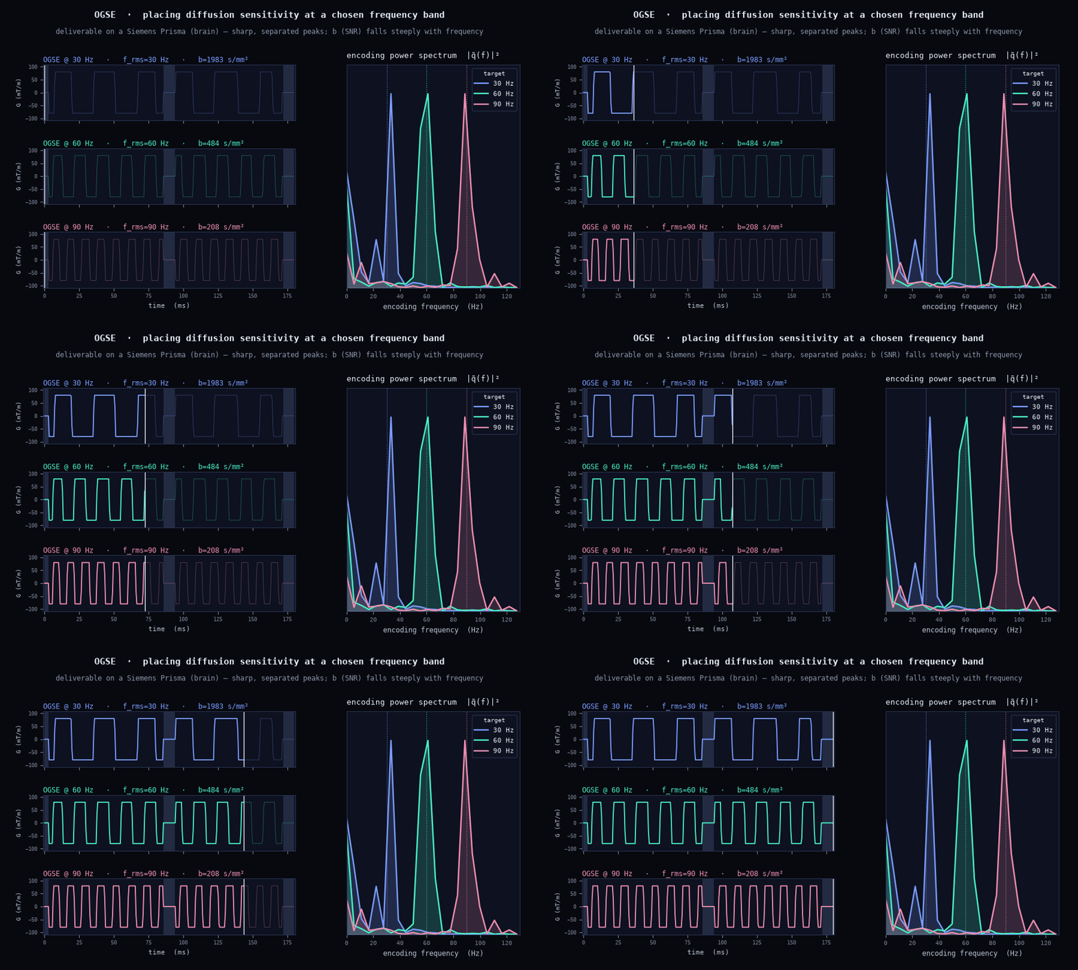
Two things to read off it. First, spectral_freq genuinely controls the encoding band — the peak sits where you ask, sharp and separated, not smeared across DC. Second, the b-value falls steeply with frequency (here 1983 → 484 → 208 s/mm² from 30 → 90 Hz): a higher encoding frequency means a shorter effective diffusion time, paid for in SNR. That trade — spectral resolution vs SNR — is the design decision OGSE forces, and the reason spectral_rms / spectral_bandwidth are reported, so you can see exactly what you bought.

Peak sharpness is set by the number of oscillation periods, N = f · T_enc. A long readout that eats the encoding time leaves only a period or two and smears the peak — which is why deliverable OGSE wants a short readout and a long TE.

Simulate and fit the same OGSE waveform

The designed OGSE waveform is an ordinary G(t), so it flows into the rest of the ecosystem with no conversion: d.to_sim_waveform() hands it to dmipy-sim for the Monte-Carlo ground-truth signal at that exact realized spectrum (spectral dispersion the b-tensor can't see included), and the same object drives the dmipy-fit analytical model — so an OGSE-aware fit is checked against the simulator on the identical acquisition, and the recovered \(D(\omega)\) is validated before any scanner time.

The full design → simulate → fit → scanner loop, and the shared free-waveform interface, are on the Run it on the scanner page.