Deliverable waveforms & constraints

Textbook diffusion MRI assumes an idealized encoding: instantaneous, infinitely sharp gradient pulses, a perfectly rectangular PGSE pair, symmetric about the 180. A real scanner can play none of that exactly. dmipy-design closes the gap — it designs the waveform a scanner can actually deliver, and the constraints below are why the realizable optimum differs from the textbook one.

Idealized vs deliverable

Idealized theory	Real hardware
instantaneous gradient switching	finite slew rate (T/m/s) and gradient raster
unbounded amplitude	maximum G (T/m)
rectangular PGSE, symmetric	encoding windows set by RF/ADC timing → often asymmetric
no physiological limits	PNS (nerve stimulation) and gradient heating caps

Asymmetric encoding windows

The 180 refocusing pulse sits at TE/2, but diffusion encoding is off during three intervals: the excitation lead-in (after the 90), the 180 itself (plus its crushers), and the readout tail (before the echo). Because the lead-in and the readout-pre-echo are generally unequal — and partial Fourier shortens the post-180 window further — the two remaining encoding windows (pre- and post-180) come out different lengths.

So the optimal waveform is asymmetric as a consequence of the timing, not as a free knob. You don't dial in "0.3 asymmetry"; you specify the physical budget (SequenceTiming, or read it from a .seq), and the asymmetry falls out. Forcing symmetry (the conventional choice) dead-times the surplus of the longer window — spins sit transverse doing nothing but losing \(T_2\) — so it encodes less b for the same TE.

See it: same b, shorter TE

Both sequences below encode the same b-value (1000 s/mm²) on the same hardware — real Siemens Prisma limits (80 mT/m, 200 T/m/s, 10 µs raster) with a realistic single-shot diffusion-EPI budget (short excitation lead-in, long EPI readout-to-echo). Both are plain monopolar bang-bang PGSE (no motion nulling — the right default for brain), so the only difference is symmetric vs asymmetric encoding. They play at the same wall-clock speed, so you can watch the optimized asymmetric design refocus first:

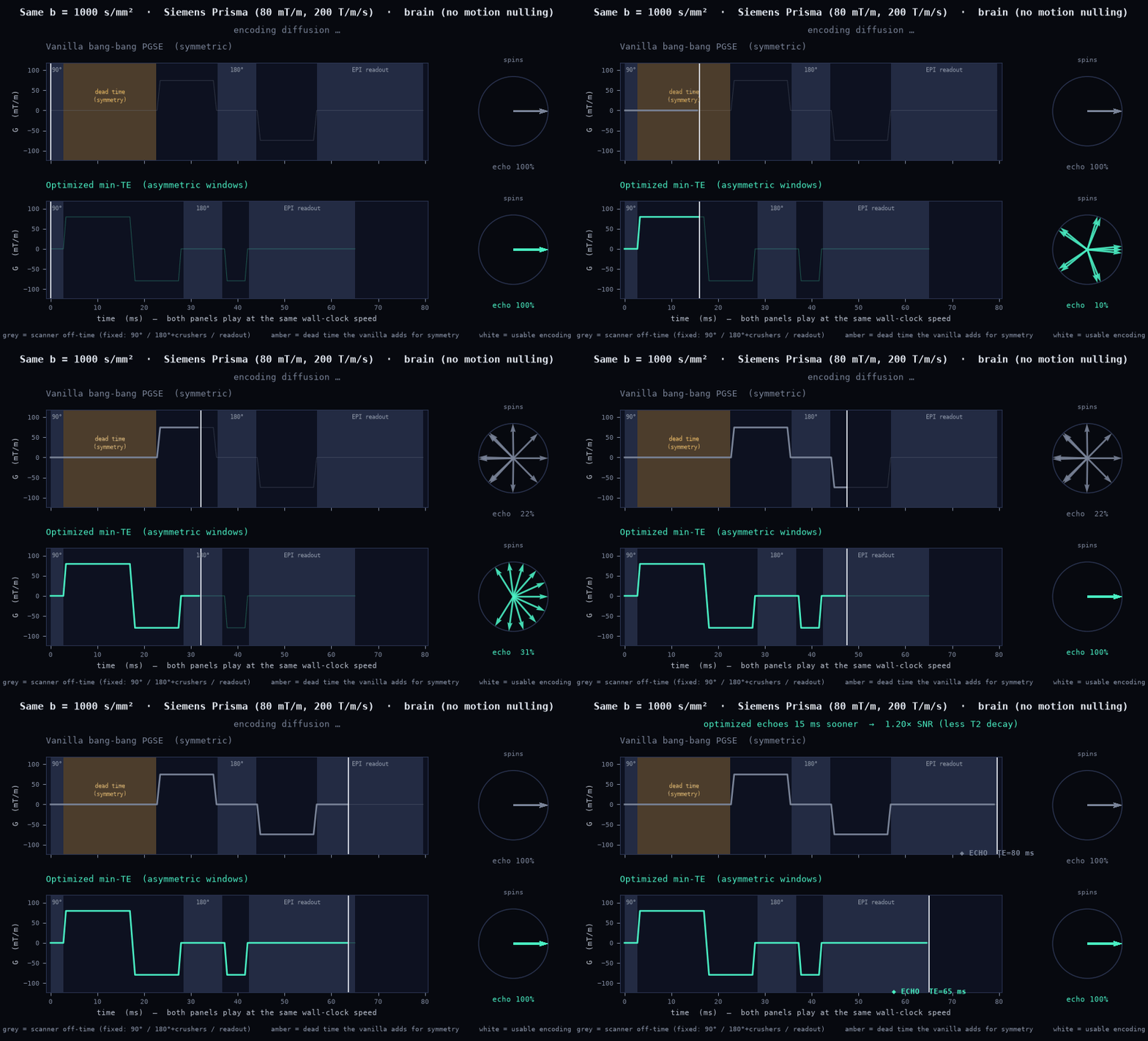
The grey bands are scanner-fixed off-times (the 90°/prep lead-in, the 180° + crushers, the EPI readout) — the hard walls of the optimization space, identical on both panels. The amber band is the extra dead time the vanilla adds purely to stay symmetric: it throws away its long pre-180 window down to the short post-180 one — that's what makes it "vanilla." The optimized design fills that same window (white = usable encoding).

So the vanilla needs TE = 80 ms; the asymmetric design reaches the same b at TE = 65 ms — 15 ms sooner, worth ≈ 1.20× SNR at \(T_2 = 80\) ms (\(e^{\Delta\mathrm{TE}/T_2}\)). Same contrast, more signal, purely from respecting the timing the scanner actually has. This is the min-TE mode at work.

The NOW constraint set — and why each exists

The NOW oracle maximises \(b = \mathbf{g}^\top \mathbf{Q}\, \mathbf{g}\) subject to the full deliverability set, each constraint enforced exactly (active-set SQP), so the b-value reaches the true realizable optimum rather than being dwarfed by penalty terms:

Constraint	Why it's there
slew |dG/dt| ≤ S_max, amplitude |G| ≤ G_max	the hardware simply cannot exceed them
refocus \(q(\mathrm{TE})=0\)	a spin echo must rephase static spins at the echo, else signal is lost
M1 / M2 nulling (velocity, acceleration)	uncompensated moments make the signal sensitive to bulk motion / flow, biasing the diffusion estimate
b-tensor shape (\(b_\Delta\))	LTE / PTE / STE encode different tissue information; the shape must be hit, not approximated
Maxwell (concomitant fields)	gradient cross-terms produce a spatially varying field that dephases signal unless nulled
spectral (RMS frequency)	OGSE-like frequency content — see OGSE spectral design
PNS (SAFE model)	see below
heat (\(\int g^2\))	duty-cycle / coil-heating budget on long protocols

When do you actually need each constraint?

The guiding principle (it's in the designer's own docstring): a needed-but-off constraint biases your measurement, while an unneeded-but-on one only costs a little b (SNR). Bias is unrecoverable; lost b is just a bit of SNR — so you default the biasing constraints on and turn one off only when its confound is physically absent. That is a per-application decision, not a global one:

Constraint	Turn it on when…	Usually off when…
M1 / M2 (motion)	body / cardiac / abdominal diffusion — pulsatile flow and bulk motion bias the signal	brain — the head is still, so plain monopolar bang-bang is standard (as in the animation above)
Maxwell (concomitant)	high gradient amplitude, off-isocenter slices, single-sided / asymmetric waveforms	time-symmetric waveforms, or near isocenter / high B0 (the term is ≈ 0 — essentially free to leave on)
spectral (OGSE)	you want frequency-resolved encoding (restriction / exchange spectroscopy)	standard PGSE — the encoding frequency is just whatever falls out
PNS, heat	effectively always — these are deliverability; at high slew / large FOV or long high-duty protocols they bind hardest	never truly off for a runnable sequence
slew, amplitude, refocus	always — the hardware and the spin echo require them	—

That is exactly why the animation above uses no moment nulling: it's a brain acquisition, the head doesn't pulse, so paying the b (and TE) cost of M1/M2 would only lose SNR to suppress a confound that isn't there. Switch to a cardiac or liver protocol and the calculus flips — the moment-nulled, non-bang-bang waveform becomes the correct one, and the constraint that was wasteful for brain is now essential.

Why PNS is a hard constraint

Rapidly switching gradients induce electric fields in the body that can stimulate peripheral nerves — an uncomfortable (and regulated) limit, not just an engineering one. Vendors accept or reject a sequence against a PNS model (the SAFE model; IEC 60601-2-33). Without a PNS constraint, a b-maximiser would happily ride the slew rate to the hardware maximum everywhere and produce a waveform the scanner refuses to run (or that stimulates the patient). dmipy-design holds PNS ≤ a target (e.g. 80 % of the stimulation limit) inside the design, so what comes out is deliverable — and pulseq_pns_report re-checks the assembled .seq with the same model the scanner uses.

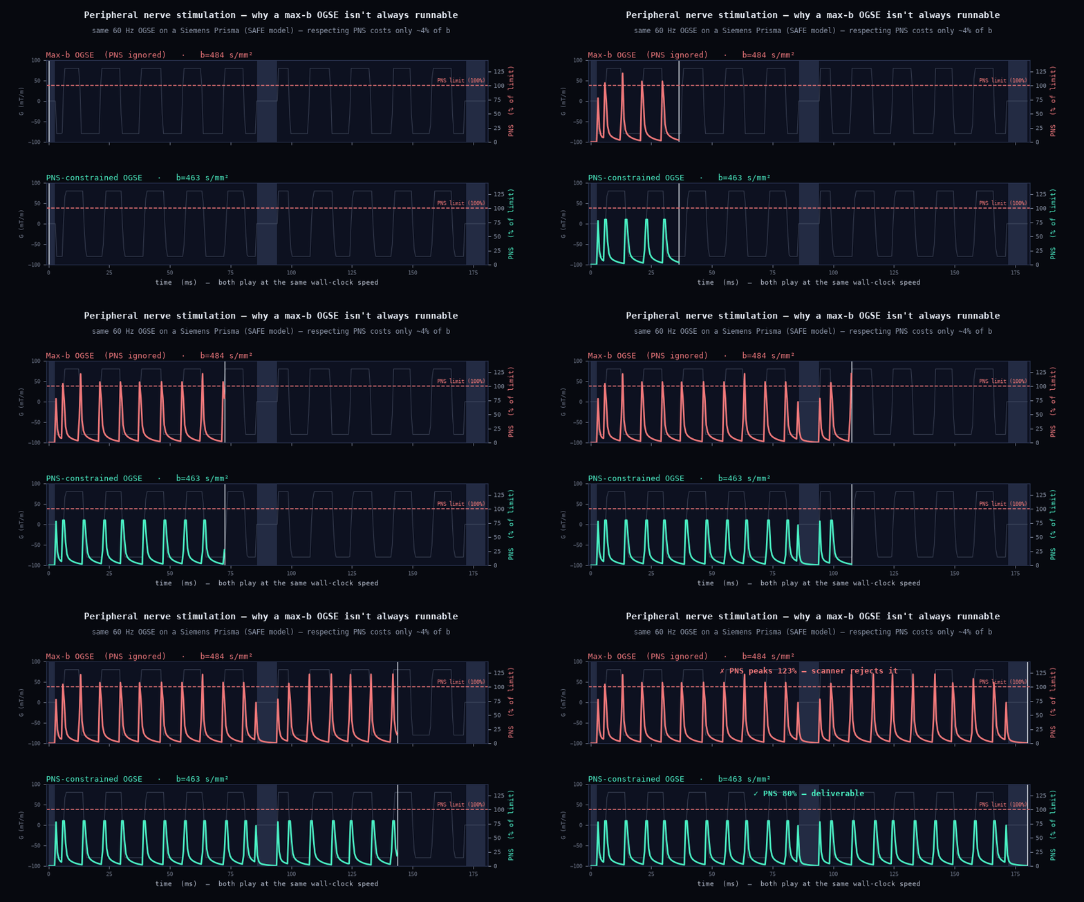
The same 60 Hz OGSE, designed with the PNS constraint off and on, makes it concrete: the max-b version rides the slew limit at every edge and peaks over the stimulation limit (the scanner would refuse it), while the constrained design stays under it for only ~4 % less b.

The payoff: it exports and passes acceptance

Because deliverability is designed in rather than checked after the fact, a design exports to a scanner-runnable Pulseq spin echo and passes the offline acceptance checks — timing, realized peak G/slew vs the system limits, and a b-tensor round-trip (what you asked for == what the assembled sequence actually encodes).