Gaussian-Phase cylinder for arbitrary waveforms
Derivation note for C4CylinderGaussianPhaseApproximation
(dmipy_fit.signal_models.cylinder_models) — the Gaussian-Phase-Approximation (GPA) cylinder
generalised from fixed-direction PGSE (Van Gelderen) to arbitrary rotating / tensor-valued
gradient waveforms (OGSE, LTE / PTE / STE, free \(\mathbf G(t)\)).
The useful result. In the fast-eigenmode limit, the perpendicular attenuation of a dispersed cylinder population depends on the waveform only through the \(l \le 2\) angular power spectrum of \(\mathbf G(t)\) (six numbers \(\Gamma_{lm}\)) plus the b-tensor — a compact, differentiable, \(O(n_t)\) closed form evaluated as a spherical-harmonic inner product against the ODF. That is what makes it cheap enough to sit inside a waveform-design loop.
Scope & honesty. This is the fast-eigenmode (long-time) approximation: accurate for radii
\(R \lesssim 3\,\mu\)m and gradient spectra below the first cylinder eigenmode; large radii and
high-frequency OGSE need the full spectral GPA. The exact result for an arbitrary waveform is
Grebenkov's multiple-correlation-function matrix formalism — this note is a fast approximation
for the restricted regime it targets, not a replacement for that. It is validated against
dmipy-sim Monte-Carlo (§6); that agreement is a consistency check between the two engines, not
an independent proof.
1. Problem statement
The classic Gaussian Phase Approximation (GPA) for a cylinder was derived for Pulsed Gradient Spin Echo (PGSE) with a fixed gradient direction. We extend it to arbitrary free-gradient waveforms \(\mathbf G(t) \in \mathbb R^3\), including rotating and tensor-valued encodings (STE, OPTICUBE21, NOW-STE, arbitrary OGSE), while preserving exact equivalence with the PGSE formula in the fixed-direction limit.
2. Physics
2.1 Accumulated phase for a single water molecule
where \(\gamma = 2.675\times10^{8}\) rad/(s·T) is the water gyromagnetic ratio, \(\mathbf G(t)\) is the gradient waveform (T/m), \(\mathbf r(t)\) the molecule position (m), and \(T\) the total waveform duration.
2.2 GPA signal for a cylinder with axis \(\hat{\mathbf n}\)
Under the Gaussian Phase Approximation the signal is
2.3 Parallel contribution (Gaussian, exact for any waveform)
where \(\mathbf B\) is the b-tensor. For PGSE, \(\mathbf B = b\,\mathbf n\otimes\mathbf n\) (rank-1), so \(\phi_\parallel = b\,(\hat{\mathbf n}\cdot\mathbf n)^2\lambda_\parallel\). For a spherical b-tensor (STE), \(\mathbf B = (b/3)\,\mathbf I\), so \(\phi_\parallel = (b/3)\lambda_\parallel\) (orientation-independent).
2.4 Perpendicular contribution: fast-eigenmode GPA
For a cylinder of radius \(R\) with impermeable wall and perpendicular diffusivity \(D\), the perpendicular phase variance in the fast-eigenmode limit is
with
- \(\mu_k\) = \(k\)-th zero of \(J_1'(x)\) (\(\mu_1 = 1.84118\), \(\mu_2 = 5.33144\), …),
- \(B_k = 2(R/\mu_k)^2 / (\mu_k^2 - 1)\) (eigenmode amplitude weights),
- \(\alpha_k = (\mu_k/R)^2 D\) (eigenmode decay rates, s⁻¹).
Validity condition: \(\alpha_k T \gg 1\), i.e. the waveform duration \(T\) must greatly exceed the eigenmode decay time \(\tau_1 = R^2/(\mu_1^2 D)\).
| \(R\) (µm) | \(D\) (m²/s) | \(\tau_1\) (ms) | Clinical \(T=75\) ms → \(\alpha_1 T\) |
|---|---|---|---|
| 1 | \(1.7\times10^{-9}\) | 0.17 | 440 (error < 0.1 %) |
| 2 | \(1.7\times10^{-9}\) | 0.69 | 109 (error < 0.1 %) |
| 5 | \(1.7\times10^{-9}\) | 4.3 | 17 (error ~ 3 %) |
2.5 Factorisation via the angular power spectrum
Using \(|\mathbf G_\perp|^2 = |\mathbf G|^2 - (\mathbf G\cdot\hat{\mathbf n})^2 = |\mathbf G|^2\,(1 - (\hat{\mathbf G}\cdot\hat{\mathbf n})^2)\), with \(\hat{\mathbf G} = \mathbf G/|\mathbf G|\),
The second integral is the \(l=2\) projection of the angular power spectrum \(\Gamma_{lm} = \int|\mathbf G(t)|^2\,Y_{lm}(\hat{\mathbf G}(t))\,dt\) onto \(\hat{\mathbf n}\). By the SH addition theorem,
so
where \(\Gamma_{2m}\) are the five \(l=2\) (\(m = -2,-1,0,1,2\)) real SH components of the gradient angular power spectrum, \(\Gamma_{2m} = \int_0^T |\mathbf G(t)|^2\,Y_{2m}(\hat{\mathbf G}(t))\,dt\), and \(\Gamma_{00} = \int|\mathbf G|^2\,dt / \sqrt{4\pi}\).
2.6 Complete single-fibre signal
This uses only two waveform-derived objects (\(\Gamma_{lm}\) and \(\mathbf B\)) and the cylinder geometry factor \(C_{\mathrm{geom}}\); both are precomputed once per measurement at \(O(n_t)\) cost.
3. Implementation algorithm
(pseudocode — the runnable model is C4CylinderGaussianPhaseApproximation.)
Step 1 — precompute \(C_{\mathrm{geom}}\) (once per \((R, D)\) pair)
Input: R (m), D (m^2/s), roots mu_k = zeros of J1'(x) (at least 100 terms)
C_geom = gamma^2 * sum_k  2(R/mu_k)^2 / (mu_k^2 - 1)  /  ((mu_k/R)^2 * D)
Step 2 — compute Gamma_lm from G(t) (shape: (n_m, 6))
Input: G[m, t, 3] in T/m, dt (s)
For each measurement m:
    Ghat[t] = G[m,t] / |G[m,t]|        (unit direction; skip t where G = 0)
    G2[t]   = |G[m,t]|^2
    (x, y, z) = Ghat[t]

    Gamma_00[m]  = sum_t G2[t] * Y00  * dt     Y00  = 1/sqrt(4 pi)
    Gamma_2m2[m] = sum_t G2[t] * Y2m2 * dt     Y2m2 = sqrt(15/4pi)  * x*y
    Gamma_2m1[m] = sum_t G2[t] * Y2m1 * dt     Y2m1 = sqrt(15/4pi)  * y*z
    Gamma_20[m]  = sum_t G2[t] * Y20  * dt     Y20  = sqrt(5/16pi)  * (2z^2 - x^2 - y^2)
    Gamma_2p1[m] = sum_t G2[t] * Y2p1 * dt     Y2p1 = sqrt(15/4pi)  * x*z
    Gamma_2p2[m] = sum_t G2[t] * Y2p2 * dt     Y2p2 = sqrt(15/16pi) * (x^2 - y^2)
Step 3 — compute the b-tensor B (shape: (n_m, 3, 3))
q[m, t] = gamma * cumsum_{t' <= t} G[m, t'] * dt    (shape (n_m, n_t, 3))
B[m, i, j] = sum_t q[m, t, i] * q[m, t, j] * dt
For PGSE, reconstruct \(\mathbf B = b\,\mathbf n\otimes\mathbf n\) analytically (avoid discretisation).
Step 4 — evaluate \(E(\hat{\mathbf n})\) for a specific fibre direction
phi_perp = C_geom * (2/3 * Gamma_00[m] * sqrt(4 pi)  -  8 pi/15 * Gamma_2m[m] . Y2m(nhat))
phi_par  = lambda_par * (nhat^T B[m] nhat)
E[m]     = exp(-phi_perp - phi_par)
Step 5 — dispersed signal via SH inner product
For an ODF \(\mathrm{ODF}(\hat{\mathbf n})\) with SH coefficients \(f_{lm}\) (Tournier/MRtrix real SH, even \(l\) only):
a. Evaluate E_m(nhat_q) at N_q = 724 quadrature points on the sphere (weights w_q = 1/724)
b. Project to SH:  E_lm[m] = 4 pi * sum_q w_q * E_m(nhat_q) * Y_lm(nhat_q)
c. Dispersed signal: S[m] = E_lm[m] . f_lm   (inner product)
The quadrature is over the full sphere (antipodally symmetric for any axis). \(l_{\max}=8\) is required: the exponent \(\exp(-\phi)\) generates harmonic content up to \(l=8\) for physically relevant parameters (\(C_{\mathrm{geom}}\,b \sim 0.1\)–\(10\)).
4. SH convention
Real symmetric SH (Tournier/MRtrix convention):
Array layout: even orders \(l = 0, 2, 4, \dots, l_{\max}\); all \(m \in [-l, l]\) per order. Total coefficients for \(l_{\max}=8\): \(1+5+9+13+17 = 45\); the \(m=0\) indices are \(l{=}0\to0\), \(l{=}2\to3\), \(l{=}4\to10\), \(l{=}6\to21\), \(l{=}8\to36\).
ODF normalisation. For any properly normalised ODF, \(f_{00} = 1/(2\sqrt\pi)\), so the dispersed signal at \(b=0\) equals 1: \(S = E_{lm}\!\cdot\! f_{lm} = 1\).
Watson ODF. Use GL quadrature (not sphere-grid fitting) for accuracy at \(\kappa \ge 20\);
dmipy_sim.sh_convolution.watson_odf_sh(kappa, lmax=8) provides accurate coefficients.
5. Key identities
PGSE limit. For a fixed-direction PGSE along \(\mathbf n\) with pulse parameters \((\delta, \Delta)\),
and \(\Gamma_{20}\) depends on \(\mathbf n\) relative to the \(z\)-axis. Then \(E(\hat{\mathbf n})\) reduces to the Van Gelderen PGSE formula when \(\delta \gg \tau_1 = R^2/(\mu_1^2 D)\).
STE (spherical b-tensor). \(\mathbf B = (b_{\mathrm{tr}}/3)\,\mathbf I_3\); the dispersed signal is ODF-independent for any anisotropic ODF because \(\mathbf u^{\mathsf T}\mathbf B\,\mathbf u = b_{\mathrm{tr}}/3\) for all \(\hat{\mathbf n}\).
Zero b-value. \(\mathbf B = 0 \Rightarrow \phi_\perp = \phi_\parallel = 0 \Rightarrow E(\hat{\mathbf n}) = 1\) for all \(\hat{\mathbf n} \Rightarrow S = 1\). ✓
6. Monte-Carlo validation
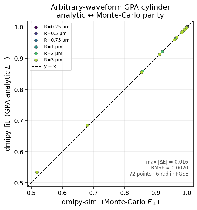
The analytical GPA cylinder (dmipy-fit) reproduces the dmipy-sim Monte-Carlo signal to within
Monte-Carlo noise across six radii (\(0.25\)–\(3\,\mu\)m) and the physiological b-range — every point
falls on the identity line (max \(|\Delta E| = 0.016\), RMSE \(0.002\)). This is the consistency check
between the two engines described in the scope note above, not an independent proof.
Validated at atol \(\le 0.02\) (\(b < 3000\) s/mm²) and atol \(\le 0.05\) (\(b \ge 3000\) s/mm²) against 500 000-walker MC trajectories for:
| Waveform | Type | Duration | \(G_{\max}\) levels (T/m) |
|---|---|---|---|
| OPTICUBE21 | STE | 100 ms | 0.05, 0.08, 0.10, 0.20, 0.30 |
| NOW-STE | STE | 75.6 ms | 0.05, 0.08, 0.10, 0.20, 0.30 |
| PGSE | linear | \(\delta{=}20\) ms, \(\Delta{=}40\) ms | 0.05, 0.08, 0.10, 0.20, 0.30 |
Radii \(R \in \{1.0, 2.0, 3.0, 5.0\}\,\mu\)m; Watson \(\kappa \in \{1, 5, 20, 100\}\). Tests (public):
dmipy_fit/signal_models/tests/test_gaussian_phase.py, test_gamma_lm_cylinder.py,
test_cylinder_fixture_ogse_dispersed.py; MC fixtures are generated and checked within that
suite. The MC uses the same SH convolution as dmipy-sim (GL fibre-response fit → apply_odf).
7. Known limitations
- Fast-eigenmode condition — error grows as \(\tau_1/T\) increases. For \(R=5\,\mu\)m, \(T=40\) ms: \(\tau_1/T = 0.11 \Rightarrow\) error ~12 % at moderate \(b\); \(R \gtrsim 3\,\mu\)m requires the full spectral GPA.
- High-frequency OGSE — when \(f > \alpha_1/(2\pi) \sim D\mu_1^2/(2\pi R^2)\) the fast-eigenmode approximation breaks. For \(R=2\,\mu\)m, \(D=1.7\times10^{-9}\): \(f_{\max} \approx 230\) Hz.
- Exchange / permeability — assumes an impermeable membrane.
- \(l_{\max}=4\) for \(\Gamma_{lm}\) — the angular power spectrum needs only \(l=0\) and \(l=2\) because the cylinder GPA involves only \(\int|\mathbf G_\perp|^2\,dt\), which projects onto \(l\le2\); higher \(\Gamma_{lm}\) orders contribute only through waveform self-products, which vanish under the fast-eigenmode limit. The SH projection of \(\exp(-\phi)\) to \(E_{lm}\) uses \(l_{\max}=8\).