Canonical white matter: the analytical model and the Monte-Carlo simulator agree
The point of dmipy-fit (analytical signal models) and dmipy-sim (Monte-Carlo of spins
under a real G(t)) is that they consume one physical substrate + sequence. This page
builds the canonical white-matter substrate, evaluates the signal both ways — the
analytical forward from dmipy-fit, and the Monte-Carlo forward from dmipy-sim — and shows
they agree, for diffusion and for surface relaxivity, both ON and OFF.
What agreement here does and does not mean
The two engines share the same Substrate/Sequence definition (fit's AcquisitionScheme
delegates to sim; the white-matter parameters are the sim biophysical catalogue). Agreement
is therefore the interface contract working — necessary, but not a proof of
correctness: the engines are correlated and could be wrong in the same way. The independent
correctness checks are the against-exact-analytics validations in
dmipy-sim/examples/validation/.
Every physical value comes from the single source of truth — the dmipy-sim biophysical
catalogue — so the two engines cannot drift apart:
import numpy as np
from dmipy_sim.substrate.biophysical_constants import canonical_white_matter
C = canonical_white_matter(3.0)
print("D_intra=%.2e  g_ratio=%.2f  rho=%.2e  T2_intra=%.3f  myelin_water_proton_density(catalogue)"
      % (C['D_intra'], C['g_ratio'], C['rho2'], C['T2_intra']))
The Monte-Carlo forward (dmipy-sim), from the base API + factory
The MC substrate is a packed myelinated-cylinder geometry built from the same catalogue Gamma
calibre distribution, g-ratio and packing fraction; the signal is simulate() over the shared
waveform. Because the sub-micron walk must be step-resolved (fine dt, step ≪ fibre) it
is run on a GPU and cached here — regenerate with python generate_mc_reference.py:
# (run in generate_mc_reference.py; shown for transparency)
from dmipy_sim import pack_myelinated_cylinders, PackedMyelinatedCylinders, simulate, pgse, set_b
inner, gr, cen = pack_myelinated_cylinders(inner_radii=g*d_out/2, g_ratios=..., target_packing=f_axon)
geom = PackedMyelinatedCylinders(inner_radii=inner, g_ratios=gr, centers=cen, cell_size=cell,
                                 D_intra=D, D_extra=D, T2_intra=..., rho_inner=rho, rho_outer=rho, ...)
S_mc = simulate(N_walkers, waveform=wf, geometry=geom, seed=1)   # step-resolved
ref = np.load('flagship_mc_reference.npz') # cached MC (generate_mc_reference.py)
The analytical forward (dmipy-fit), from the base API + factory
The analytical model is an ordinary MultiCompartmentModel assembled from standard
compartments by the white-matter factory. lambda_perp is the fibre-fraction tortuosity
constraint (a dependent parameter, not free); myelin is water-weighted by the catalogue
myelin_water_proton_density. We evaluate it live on the same acquisition scheme:
from dmipy_fit.white_matter.composition import build_white_matter_model
from dmipy_fit.core.acquisition_scheme import acquisition_scheme_from_bvalues

bvals, bvecs, TE = ref['bvals'], ref['bvecs'].astype(float), float(ref['TE'])
scheme = acquisition_scheme_from_bvalues(bvals, bvecs, delta=float(ref['delta']),
                                         Delta=float(ref['DELTA']), TE=TE)

def analytic(rho):
    model, p = build_white_matter_model()          # tortuosity constraint on by default
    p = dict(p); p['OccupancyGatedModel_1_mu'] = np.array([0.0, 0.0])   # fibre along z
    p['OccupancyGatedModel_1_surface_relaxivity'] = rho
    p['OccupancyGatedModel_2_surface_relaxivity'] = rho
    return np.asarray(model(scheme, **p)).ravel()

S_fit_diff = analytic(0.0)
(1) Diffusion signal — the two engines agree
S_mc_diff = ref['S_mc_diff']
fit_n, mc_n = S_fit_diff / S_fit_diff[0], S_mc_diff / S_mc_diff[0]
labels = ['b0', 'b1‖', 'b2‖', 'b1⊥', 'b2⊥']
for l, a, b in zip(labels, fit_n, mc_n):
    print(f"  {l:>4}:  fit {a:.3f}   mc {b:.3f}   Δ {abs(a-b):.3f}")
gap = float(np.max(np.abs(fit_n - mc_n)))
print("max diffusion gap:", round(gap, 3))
assert gap < 0.06, f"diffusion parity gap {gap:.3f} exceeds small-N tolerance"
(2) Surface relaxivity — it matters, and both engines agree ON and OFF
Surface relaxivity shortens the apparent T₂, dropping the b=0 signal. The analytical
IntraPoreSurfaceRelaxivity/ExteriorSurfaceRelaxivity factors and the MC's wall relaxivity
rho_inner/rho_outer are the same physics on the same S/V:
S0_fit_off, S0_fit_on = float(analytic(0.0)[0]), float(analytic(C['rho2'])[0])
S0_mc_off, S0_mc_on = float(ref['S0_mc_surf_off']), float(ref['S0_mc_surf_on'])
print(f"  surface OFF:  fit S0 {S0_fit_off:.3f}   mc {S0_mc_off:.3f}   Δ {abs(S0_fit_off-S0_mc_off):.3f}")
print(f"  surface ON :  fit S0 {S0_fit_on:.3f}   mc {S0_mc_on:.3f}   Δ {abs(S0_fit_on-S0_mc_on):.3f}")
drop = 1 - S0_fit_on / S0_fit_off
print(f"  surface term removes {100*drop:.0f}% of S0  (non-trivial)")
assert abs(S0_fit_off - S0_mc_off) < 0.02 and abs(S0_fit_on - S0_mc_on) < 0.02
assert drop > 0.10, "surface effect should be a sizeable fraction of the signal"
import matplotlib
matplotlib.use("Agg")
import matplotlib.pyplot as plt
fig, ax = plt.subplots(1, 2, figsize=(8.2, 3.4))
x = np.arange(len(labels))
ax[0].plot(x, fit_n, 'o-', label='analytical (dmipy-fit)')
ax[0].plot(x, mc_n, 's--', label='Monte Carlo (dmipy-sim)')
ax[0].set_xticks(x); ax[0].set_xticklabels(labels); ax[0].set_ylabel('S / S(b0)')
ax[0].set_title('Diffusion signal'); ax[0].legend(fontsize=8); ax[0].grid(alpha=0.3)
ax[1].bar([0, 1], [S0_fit_off, S0_fit_on], width=0.35, label='analytical')
ax[1].bar([0.4, 1.4], [S0_mc_off, S0_mc_on], width=0.35, label='Monte Carlo')
ax[1].set_xticks([0.2, 1.2]); ax[1].set_xticklabels(['surface OFF', 'surface ON'])
ax[1].set_ylabel('S0'); ax[1].set_title('Surface relaxivity'); ax[1].legend(fontsize=8)
fig.tight_layout(); fig.savefig('canonical_wm_parity.png', dpi=130, bbox_inches='tight')
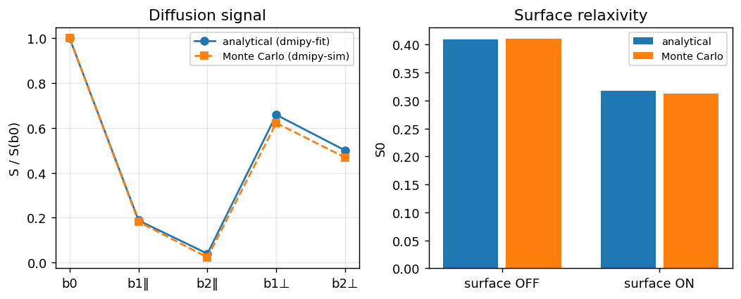
Both panels: the analytical model and the Monte-Carlo simulator, built from one substrate, land on top of each other — for diffusion and for surface relaxivity, in both states — with the surface term removing a clearly non-trivial slice of signal.
The runnable notebook lives in the dmipy-fit repo: examples/flagship_canonical_wm/.